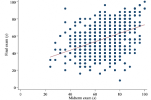
In the most common form, the estimated coefficients denote the change in the average value of the dependent variable, given a one-unit increase in the independent variable, holding other variables fixed. In the example of students’ scores for their final and midterm test (see figure below), the idea is illustrated by means of the red line that is drawn through the cloud of points. Specifically, a one-point increase for the midterm test is associated with a 0,5 point increase in the average value for the final test.

If the independent variable is a 1/0 variable (for example, whether the law student is an exchange student or not), the coefficient captures the difference in the average value of the dependent variable between both groups that are indicated by the 1/0 variable.

Testing

Academic papers usually include “regression tables”. Each coefficient is listed together with its standard error, which reflects the uncertainty around the estimated coefficient. In the end, the researcher is interested in whether the coefficient equals zero (the null hypothesis), indicating no relationship between the dependent and independent variable, or not. The estimated coefficient is divided by its standard error (uncertainty), known as the t-value or t-ratio, to determine whether the estimate is statistically different from zero. If this t-ratio is high enough in absolute sense – meaning that the coefficient is estimated with relatively high certainty and relatively distant from zero – the estimate is said to be significantly different from zero. In that case, there is a significant relationship between the dependent variable and the independent variable.

Logarithms

In some applications the dependent variable appears in logarithmic form. This can be done to reduce the tails of the distribution of the dependent variable, and to better fulfil the distributional assumptions. In case the dependent variable is in logarithms, then the coefficient informs us about the percentual change in the dependent variable given a one-unit increase in the independent variable. There are four possibilities in total, and these are shown in the table below. For example, if the logarithm is also taken of the independent variable, then the coefficient captures the percentual change in the dependent variable given a one-percent increase in the independent variable.

Model	Dependent variable	Independent variable	Interpretation of coefficient
Level-level	y	x	∆y=β∆x
Level-log	y	log(x)	∆y=(β/100)%∆x
Log-level	log(y)	x	%∆y=(100β)∆x
Log-log	log(y)	log(x)	%∆y=β%∆x

Source: Wooldridge (2016), Table 2.3. Log(·) denotes the natural logarithm.